A first speed controller

P and PI control, voltage saturation and integrator anti-windup.

Why add external feedback?

Back EMF reduces load sensitivity but does not restore a commanded speed. A controller compares reference r with measured speed and adjusts voltage. Use r = 60 rad/s, voltage limits ±12 V and a 0.1 N·m load step at 1 s. Sensors and the converter are ideal here; practical current limits, sampling and delays come later.

Proportional control

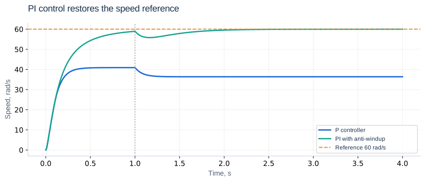
A nonzero voltage is needed to sustain speed, so a pure P controller normally needs a nonzero error. Raising Kp reduces the error but can make transients more aggressive and cannot remove actuator limits. With Kp = 0.3 and r = 60, the unsaturated no-load equilibrium is about 40.91 rad/s.

Integral action and feasibility

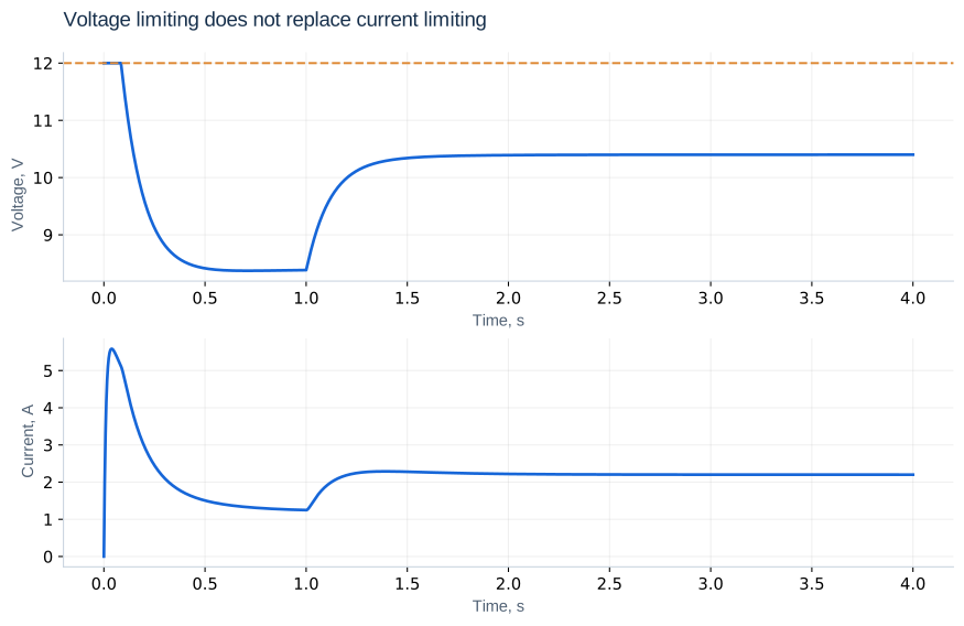
In a stable unsaturated equilibrium with constant reference, z′ = 0 implies zero speed error. Use Kp = 0.3 V·s/rad and Ki = 1 V/rad as teaching values, not universal settings. At 60 rad/s with a 0.1 N·m load, required current is 2.2 A and voltage 10.4 V, so the reference is feasible. At 100 rad/s it requires 16 V; no gain can make a 12 V actuator achieve it.

Saturation and windup

error = target - speed
raw = kp*error + ki*z
voltage = np.clip(raw, -12, 12)
outward = ((raw >= 12 and error > 0) or
           (raw <= -12 and error < 0))
dz = 0.0 if outward else error

Conditional integration stops accumulation when the error pushes further into saturation and resumes when it helps leave the limit. Voltage limiting is not current limiting. Inspect current and saturation duration as well as speed quality.

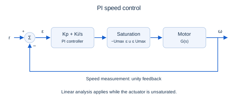
Reference and disturbance channels

These transfer functions describe the linear unsaturated regime. The integral term increases low-frequency gain, but does not make an unreachable reference reachable.

Full-model PI stability

For a positive leading coefficient, a cubic is Hurwitz when all coefficients are positive and a₂a₁ > a₃a₀. With positive gains, the displayed bound remains. At Kp = 0.3, Ki < 44.44 V/rad. Ki = 1 satisfies it, but stability alone guarantees neither acceptable overshoot nor current. The boundary is not a recommended tuning point.

An initial reduced-model tuning

Choosing ζ = 0.8 and ωn = 5 rad/s gives Kp = 0.18 and Ki = 1. Validate this initial tuning on the full model. A PI zero changes the closed-loop numerator, so the standard no-zero second-order overshoot formula is not exact here.

Back-calculation and validation

Back-calculation returns the integral voltage state toward a realizable command. A very small Tt introduces a fast scale requiring finer integration. Compare it with conditional integration under identical limits. Test small and large reference steps, load application and removal, an unreachable reference followed by a reduction, and R/J changes of ±20%.

Independent exercises

1. For Kp = 0.18, find the full-model Ki limit. Is Ki = 40 stable?

2. At r = 60 rad/s, ML = 0.1 N·m and Ki = 1, find equilibrium z.

Practical work

Compare Kp = 0.15, 0.3, 0.6 with Ki = 1, then Ki = 0.5, 1, 2 with Kp = 0.3. Tabulate settling time with a stated band, peak current, overshoot, disturbance dip and saturation duration. Compare protected and unprotected integration when a 100 rad/s reference drops to 40 rad/s.

Calculated illustrations

Key takeaways

Use feasibility, linear stability and nonlinear experiments together. The next lessons extend the model to identification, PWM, cascaded control, flexible mechanics and digital control.