The mathematics of change
Derivatives, integrals, initial-value problems and the connection between poles and responses.
Before you begin: derivatives, integrals, complex numbers and quadratic equations.
After this lesson you can: solve a linear initial-value problem and retain initial conditions in the Laplace transform.
Work through the explanation, examples, practical experiment and independent exercises.
A derivative is a rate of change
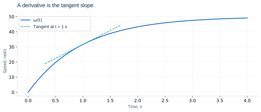
If rotor speed increases by 4 rad/s in 0.2 s, average acceleration is 20 rad/s². The derivative is the limiting rate over a short interval. A horizontal speed trace has nearly zero acceleration; a steep upward trace has large positive acceleration. Zero speed does not imply zero acceleration.
An integral accumulates change
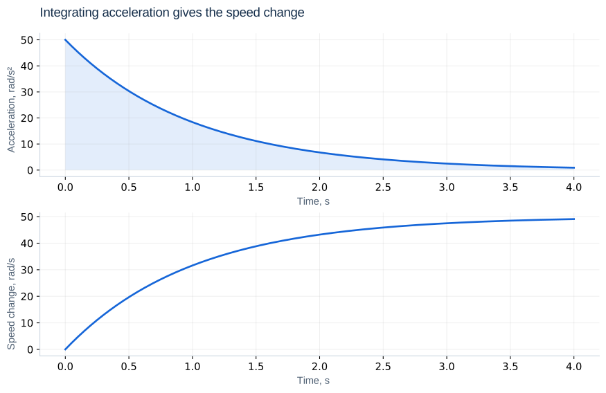
At a constant acceleration of 10 rad/s² for 0.3 s, speed increases by 3 rad/s. If ω₀ = 5 rad/s, the result is 8 rad/s. An integral is a signed area: negative acceleration subtracts speed. Integrating current gives charge, and integrating power gives energy. Units provide a useful check: W·s = J.
From a physical law to an equation
With constant applied torque and viscous friction, the current speed determines its own slope. Increasing speed raises friction and reduces acceleration until M = bω. A numerical solver follows these local slopes without knowing ω(t) beforehand. An initial condition such as ω(0) = 0 selects starting from rest; the equation alone describes many possible motions.
The state vector
For a motor, collect current and speed as y = [i, ω]. The right-hand side receives both states and returns their derivatives in the same order. Never change that order between equations, initial conditions and output interpretation.
def rhs(t, y):
    current, speed = y
    di = (12 - 2*current - 0.1*speed) / 0.02
    dw = (0.1*current - 0.002*speed) / 0.002
    return [di, dw]
These returned numbers are rates, not the next current and speed. Their units are A/s and rad/s². The solver, not this function, integrates them.
Initial conditions and the Laplace transform
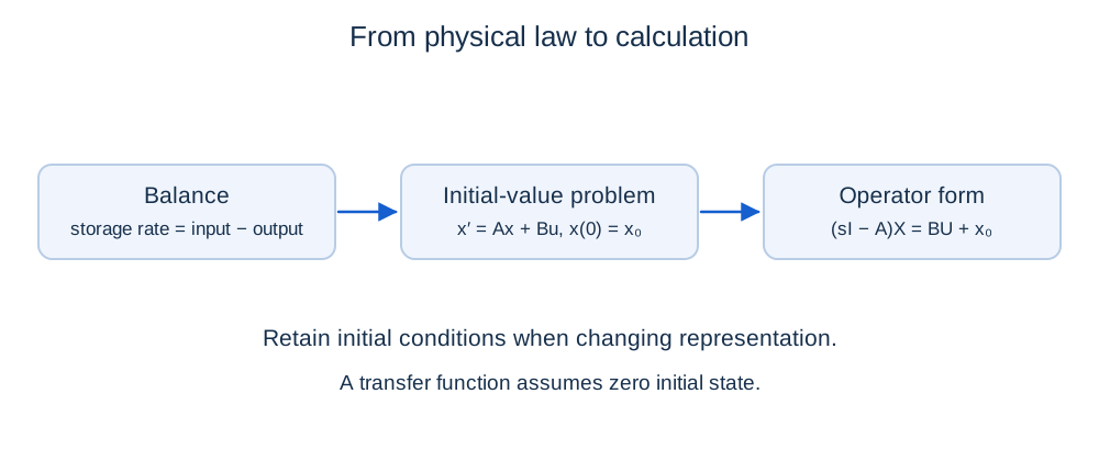
τx′ + x = Ku ⇒ X(s) = [KU(s) + τx₀]/(τs + 1)
A transfer function G(s) = K/(τs + 1) describes the input–output relation with zero initial state. Nonzero initial energy contributes a separate term. For x′ = Ax + Bu, the operator equation is (sI − A)X = BU + x₀. With constant inputs and an existing equilibrium, x(t) = x∞ + exp(At)(x₀ − x∞).
Second order: roots and motion
s₁,₂ = −ζωn ± ωn√(ζ² − 1)
For ζ > 1, the poles are distinct negative real numbers; at ζ = 1 they coincide; for 0 < ζ < 1 they are complex conjugates. The oscillatory natural response has an exp(−ζωₙt) envelope and damped frequency ωd = ωₙ√(1 − ζ²). Negative real parts produce decay; zero real parts do not give asymptotic stability.
First peak time = π/ωd
These peak formulas apply to the standard second-order system without zeros, for a unit step and zero initial conditions. They do not automatically apply to every output of a multivariable model.
Further reading: Swarthmore College: second-order poles and responses. Notation may differ from this course.
Independent exercises
1. Solve 0.2x′ + x = 5 with x₀ = 1. Find X(s), x(0.2) and x′(0⁺).
Show solution
X(s) = [5/s + 0.2]/(0.2s + 1). The solution is x = 5 − 4e⁻⁵ᵗ, so x(0.2) = 3.528 and x′(0⁺) = 20.
2. Find the poles, damping ratio, damped frequency and overshoot of x″ + 6x′ + 25x = 25u.
Show solution
ωₙ = 5 rad/s, ζ = 0.6, poles −3 ± 4j s⁻¹ and ωd = 4 rad/s. Standard step overshoot is 9.48%; the first peak occurs at 0.785 s.
Practical work
Check an analytical first-order solution by substitution and by its initial value. List the units of every derivative in the motor right-hand side. Compare real and complex pole cases. Explain why a second-order equation needs two independent initial conditions.
Calculated illustrations
Key takeaways
Derivatives describe local change and integrals accumulate it. State the variable order, derivative units and initial conditions before using a solver.
Progress is stored only in this browser.